倒産確率推定の話②

アプローチ②：オプション・アプローチ

森平（2000）*1を主に参考にして勉強しました。将来資産が将来負債額を下回る「確率」を推定する、とざっくり捉えてます。これが、コールオプションの価格決定理論に基づいているため「オプション・アプローチ」と呼ばれたりします。同論文では以下において、 $E_t,\sigma_E,\mu_D,D_T$ は所与の値で、 $\mu_A, \sigma_A, A_t$ をガウス・ザイデル法で求めるよう書いています。後述する実装例では反復回数50のガウス・ザイデル法を用いました。

$\mu_A = (\frac{E_t}{A_t})\mu_E+(1-\frac{E_t}{A_t})\mu_D\\ d_1^* \equiv \frac{ln(A_t/D_T)+(\mu_A+\sigma^2_A/2)T}{\sigma\sqrt{T}} \\ \sigma_A = \sigma_E\frac{E_t}{A_t N(d_1^*)} \\ d_2^* \equiv d_1^* - \sigma_A\sqrt{(T)} \\ A_t = \frac{E_t+D_T\cdot N(d_2^*)}{N(d_1^*)} \\$

各変数が意味するところは以下通り。

$\mu_A$ は株式価格の期待値
$\mu_E$ は負債成長率の期待値
$E_t$ は株式（自己）資本総額（株価 $\times$ 発行済み株式数）
$A_T$ は資産価値
$D_T$ は負債価値

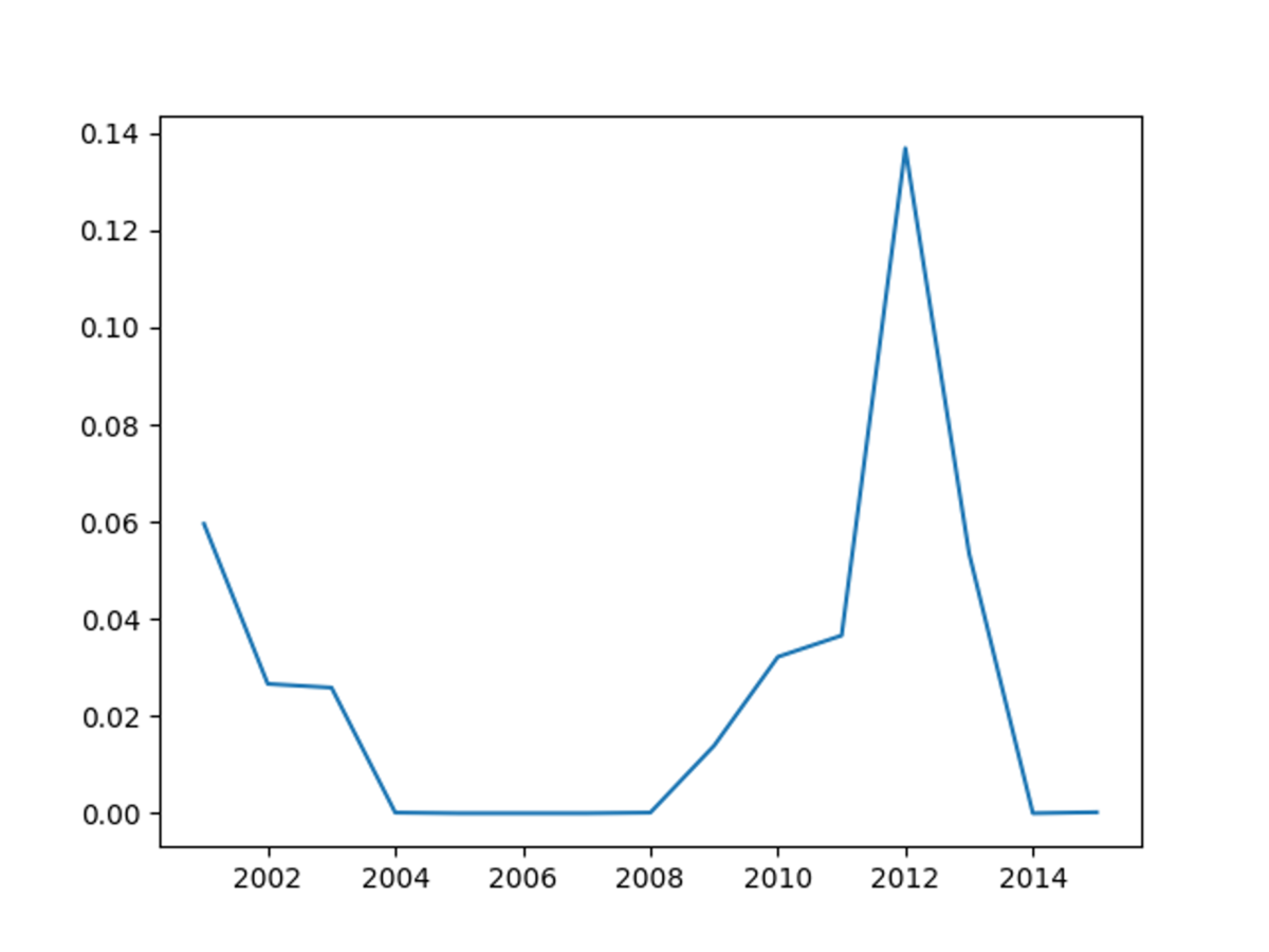
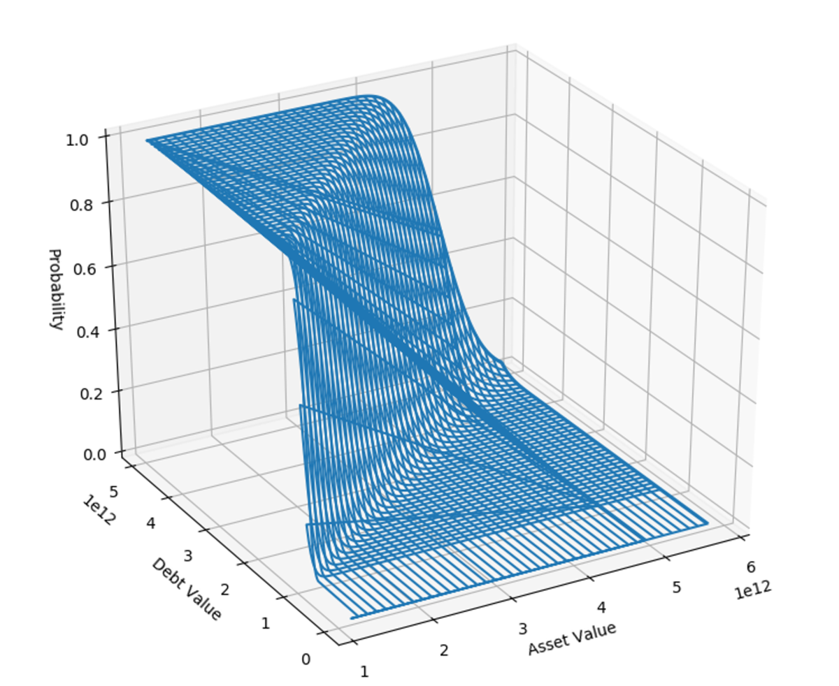
1994年から2016年までのシャープの推計を行うと以下の１枚目の画像のようになりました。実装例には含めていませんが、ある程度の幅をとってシミュレーションした結果が２枚目の画像です。

f:id:Noooooz:20211110005246p:plain — 年ごとの倒産確率の推移

f:id:Noooooz:20211110005322p:plain — シミュレーション例

シャープの財務データを使ったPythonの実装例は以下です。1994年から2016年の各変数に必要な財務データを有価証券報告書から見つけて、おそらく手作業になるけど、csvファイルにすると使えるはず。（あるいは所属大学や組織の商用データベースで。）

#This code calucurating 'Option-based Bunkruptcy risk' from time t to T=1.
#'T = 1' means 1 year later from time t.
#The Expected growth-rate of asset(= marketcapitalization) debt
#are calucurated with datas for last five years.

#Through the process below, calucurating the parameters; mu_A, sigma_A, A_t.
#Other parameters are given; E_t, sigma_E, mu_E, mu_D, D_T, T.
#The process uses Gauss-Seidel method.

#Company: SHARP

import pandas as pd
import numpy as np
from scipy.stats import norm
import math
import matplotlib.pyplot as plt


#Reading time-series data of debt and equity and maeket capitalization
#as Dataframe of Pandas
sharp_debt_pd = pd.read_csv('シャープの負債額csvの絶対パス', header = None)
sharp_equity_marketcap_pd = pd.read_csv('シャープの株式資本総額csvの絶対パス', header = None)

#Chaging datatypes of number as 'float'
sharp_debt_pd[2] = sharp_debt_pd[2].astype(float)

#Debt is given from the company's B/S, 
#so the number of figure should be fixed.
sharp_debt_pd[2] = sharp_debt_pd[2] * 1000000
print('Debt of sharp 1994-2016')
print(sharp_debt_pd)
print('-------------------------')


sharp_equity_marketcap_pd[1] = sharp_equity_marketcap_pd[1].astype(float)
sharp_equity_marketcap_pd[2] = sharp_equity_marketcap_pd[2].astype(float)
print('Market capitalization (=0) and equity price (=1) 1994-2016')
print(sharp_equity_marketcap_pd)
print('-------------------------')


#Calucurating change rates per yaer
#Changing the names of Dataframes
#Be careful of not forgetting first line would be NaN
#on 'changes_..._pd'
changes_debt_pd = pd.DataFrame()
changes_equity_marketcap_pd = pd.DataFrame()

changes_debt_pd[0] = sharp_debt_pd[2].pct_change()

changes_equity_marketcap_pd[0] = sharp_equity_marketcap_pd[1].pct_change()
changes_equity_marketcap_pd[1] = sharp_equity_marketcap_pd[2].pct_change()

final_result = list()



print('Changes of debt')
print(changes_debt_pd)
print('-------------------------')
print('Changes of market capitalization (=0) and equity price (=1)')
print(changes_equity_marketcap_pd)
print('-------------------------')



#Defining parameters gotten given from the time-series data upper at t.
for t in range(8,23):

    #'iloc' should be chosen to specify component of dataframe with number.
    #There is a explaination for it in Japanses.
    # https://yolo.love/pandas/loc-iloc-at-iat/

    #E_t is the market capitalaization at time t.
    E_t = sharp_equity_marketcap_pd.iloc[t, 1]

    #Calucurating a sigma of equity for last 5 years.
    sigma_E = changes_equity_marketcap_pd.iloc[t-5:t, 1].std()

    #Calucurating a mu of equity price change for last 5 years.
    mu_E = changes_equity_marketcap_pd.iloc[t-5:t, 1].mean()

    #Calucurating a mu of debt change for last 5 years.
    mu_D = changes_debt_pd.iloc[t-5:t, 0].mean()
    

    #D_T is amount of debt after 1 year.
    #[let a debt on book (at t = T) be regard as effectivness for 1 year]
    D_T = sharp_debt_pd.iloc[t, 2]

    #T=1 means measuring a risk of bankruptcy of 1 years later.
    T = 1
    print('E_t is ' + str(E_t))
    print('sigma_E is ' + str(sigma_E))
    print('mu_E is '+ str(mu_E))
    print('mu_D is ' + str(mu_D))
    print('D_T is ' + str(D_T))


    #Creating equation based Gauss-Seidel method 
    # with the parameters defined upper.

    #Number of times of roop to get convergence value(=answer at t) is n.
    #First, initial value should be created.

    #The initial values are be calucurated with historical data to
    #avoid a result of error caused by limitations.
    n = 50
    mu_A = np.array([0.25493648])
    sigma_A = np.array([1.24735172])
    A_t= np.array([1.348580e+12])

    #Creating a empty pd.DataFrame to show final results at each t.
    final_results = pd.DataFrame()

    
    #roop start
    for k in range(0,n+1):
        
        d_1 = (np.log(A_t[k] / D_T) + (mu_A[k] + (sigma_A[k])**2/2 ) * T) / (sigma_A[k] * np.sqrt(T))
        sigma_A_ = sigma_E * E_t / (A_t[k] * norm.cdf(x=d_1, loc=0.5, scale=1) )
        sigma_A = np.append(sigma_A, sigma_A_)

        d_2 = d_1 - sigma_A[k+1] * np.sqrt(T)
        A_t_ = (E_t + D_T * norm.cdf(x=d_2, loc=0.5, scale=1)) / norm.cdf(x=d_1, loc=0.5, scale=1)
        A_t = np.append(A_t, A_t_)

        mu_A_ = (E_t/A_t[k+1]) * mu_E + (1 - E_t/A_t[k+1]) * mu_D
        mu_A =np.append(mu_A, mu_A_)
    
    print(sigma_A[n])
    print(A_t[n])
    print(mu_A[n])
        
    

    d = (np.log(A_t[n] / D_T) + (mu_A[n] + (sigma_A[n])**2/2 ) * T) / (sigma_A[n] * np.sqrt(T))
    bankruptcy_risk_t = 1 - norm.cdf(x=d, loc=0.5, scale=1)

    print(d)
    print(bankruptcy_risk_t)
    final_result.append(bankruptcy_risk_t)
        
print(final_result)

y = final_result
x = list(range(2001, 2016))

plt.plot(x, y)
plt.show()

*1:森平爽一郎（2000）「信用リスクの測定と制御」計測と制御. （2.3 オプション・アプローチ）信用リスクの測定と制御

Noz

OR出身, 小売系データ分析

倒産確率推定の話②

アプローチ②：オプション・アプローチ